
WE4 illustrates the use of package diversity to perform variogram-based multi-scale ordinations (msov) as in Couteron & Ollier (2005). The specific functions are depend on spdep package, which must be intalled before loading diversity. The worked example uses Counami Forest Inventory data set (CFI) from Couteron et al. (2003).
1 - Data input
Once the library diversity
has been installed and loaded:
data(CFI)
str(CFI)
2 - Spatial patterns displayed by CA axes
Perform CA of the species abundance table:
cfi.ca<-ca.richness(CFI$tab,test=FALSE)
#Select the number of axes:
3
summary(cfi.ca)
#class: summary.dudiv
#metric: Richness
#call: ca.richness.default(Y = CFI$tab,
test = FALSE)
#
#total diversity: 58
#explained diversity: 5.57
#ratio of explained diversity: 0.096
Compute the k lists of neighbours
defining the scales (distance classes) of the spatial analysis:
cfi.knb<-bornes2knb(CFI$xy,c(0.38,0.45,0.80,1.20,2.00,3.00,4.00,5.00,7.00,9.00,13.00))
summary(cfi.knb)
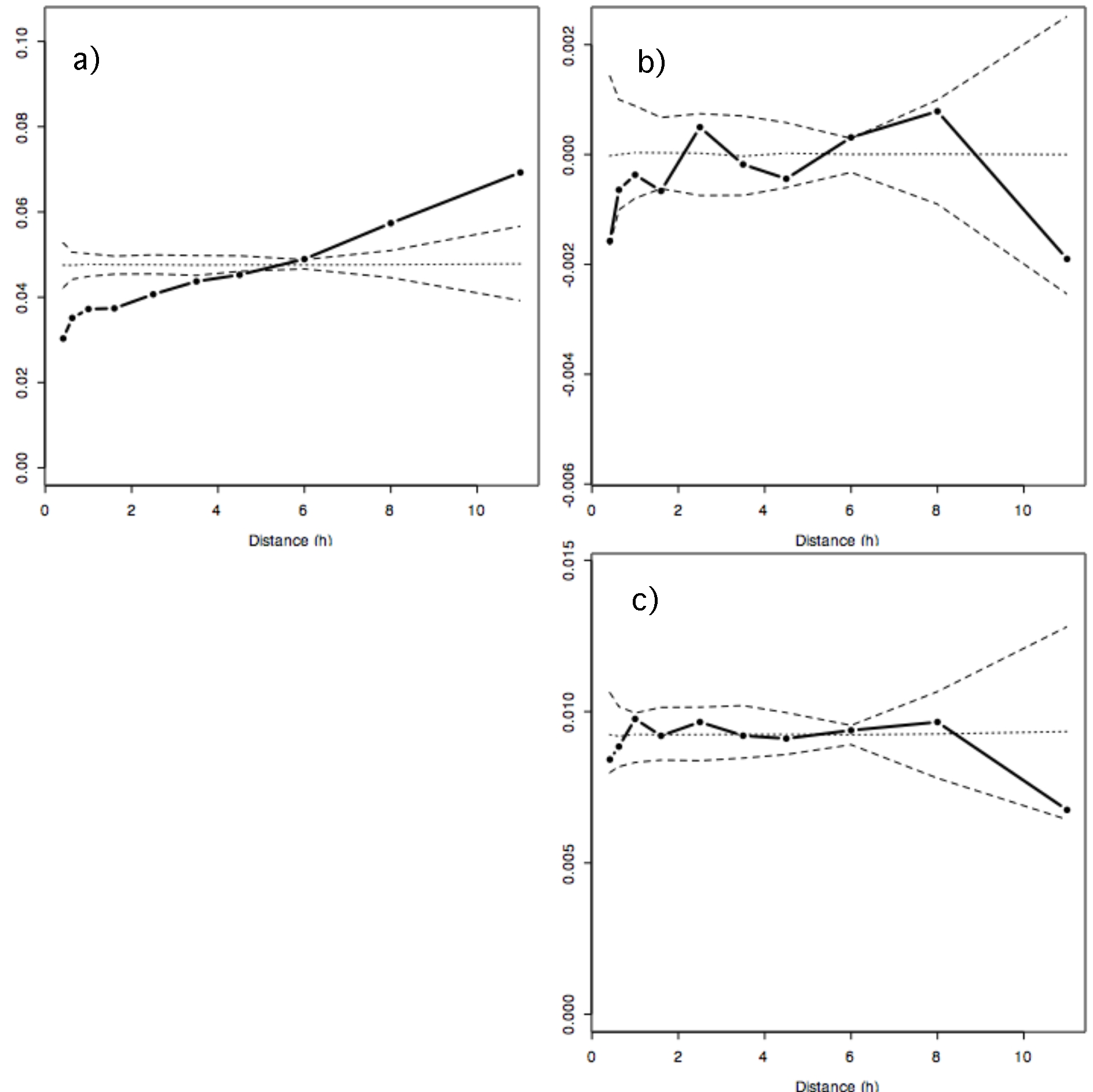
Compute the variograms and cross-variogram of CA axes 2 and 3, with tests
of statistical significance based on 300 reallocations of the floristic
compositions to the the sample sites (this could take a few minutes to
run):
cfi.ca.rtest<-kmsov.rtest(cfi.ca,cfi.knb,ax=c(2,3),nrepet=300)
a) variogram of CA axis 2 (Fig. 1a black in the original paper)
b) cross-variogram of CA axes 2 and 3 (Fig. 1e)
c) variogram of CA axis 3 (Fig. 1b black)
3 - Spatial patterns displayed by residual CA axes
Perform residual-CA of the species abundance table, once the effect of the 'topo' variable has been removed:
cfi.ca.res<-ca.richness(CFI$tab~Condition(CFI$topo),test=FALSE)Compute the variograms and cross-variogram of residual-CA axes 2 and 3,
with tests of statistical significance based on 300 reallocations of the
floristic compositions to the the sample sites (this could take a few
minutes to run):
cfi.ca.res.rtest<-kmsov.rtest(cfi.ca.res,cfi.knb,ax=c(2,3),fac=CFI$topo,nrepet=300)

4 - Spatial patterns displayed by NSCA
axes
Perform NSCA of the species abundance table:
cfi.nsca<-nsca.simpson(CFI$tab,test=FALSE)Compute the variograms and cross-variogram of NSCA axes 1 and 2, with tests
of statistical significance based on 300 reallocations of the floristic compositions
to the the sample sites (this could take a few minutes to run):
cfi.nsca.rtest<-kmsov.rtest(cfi.nsca,cfi.knb,ax=c(1,2),nrepet=300)
5 - Spatial patterns displayed by residual
NSCA axes
Perform residual NSCA of the species abundance table, once the effect of the 'topo' variable has been removed:
cfi.nsca.res<-nsca.simpson(CFI$tab~Condition(CFI$topo),test=FALSE)Compute the variograms and cross-variogram of residual-NSCA axes 1 and
2, with tests of statistical significance based on 300 reallocations of
the floristic compositions to the the sample sites (this could take a
few minutes to run):
cfi.nsca.res.rtest<-kmsov.rtest(cfi.nsca.res,cfi.knb,ax=c(1,2),fac=CFI$topo,nrepet=300)

Couteron, P., Pélissier, R. Mapaga, D., Molino, J.-F. and Teillier, L. 2003. Drawing ecological insights from a management-oriented forest inventory in French Guiana. Forest Ecology and Management, 172:89-108.
Couteron, P. and Ollier, S. 2005. A generalized, variogram-based framework
for multiscale ordination. Ecology, 86:828-834.