It illustrates the use of Diversity.R functions to perform additive diversity partitionning from Couteron & Pélissier (2004). It uses CFI data set from a 12 240-ha rainforest plot called Counami Forest Inventory (CFI) in French Guiana (Couteron et al. 2003).
1 -
Data input
Once the library diversity
has been installed and loaded:
data(CFI)
str(CFI)
#List of 4
# $ topo: Factor w/ 12 levels "10","20","21",..: 3 3 4 7 7 12 3 10 1 12 ...
# $ xy : num [1:411, 1:2] 0 0 0 0 0 0 0 0 0.5 0.5 ...
# ..- attr(*, "dimnames")=List of 2
# .. ..$ : chr [1:411] "1" "2" "3" "4" ...
# .. ..$ : chr [1:2] "X" "Y"
# $ tab : int [1:411, 1:59] 1 2 5 2 1 0 0 3 0 0 ...
# ..- attr(*, "dimnames")=List of 2
# .. ..$ : chr [1:411] "1" "2" "3" "4" ...
# .. ..$ : chr [1:59] "Sp1" "Sp2" "Sp3" "Sp4" ...
# $ dbh : int [1:411, 1:14] 6 11 5 8 9 10 8 13 7 8 ...
# ..- attr(*, "dimnames")=List of 2
# .. ..$ : chr [1:411] "1" "2" "3" "4" ...
# .. ..$ : chr [1:14] "C1" "C2" "C3" "C4" ...
CFI$tab is an abundance matrix of 59 tree species in 411 plots ;
CFI$topo is a vector of 12 eco-topographical
codes assigned to plots ;
CFI$xy is a matrix of geographical
co-ordinates of plots ;
CFI$dbh is a matrix of the frequency
distribution of trees within plots into 14 diameter classes.
2 - Nested analysis of species diversity with respect to plots and topographical
classes
Create from CFI an occurrence data frame (odf) containing the taxonomic, sampling and eco-topographical information for each individual:
CFIo<-odf(CFI$tab,CFI$topo)
str(CFIo)
#Classes
odf and `data.frame': 7189 obs. of 3 variables:
# $ tab.col : Factor w/ 59 levels "Sp1","Sp2","Sp3",..: 1 1 1 1 1 1 1 1 1
1 ...
# $ tab.row : Factor w/ 411 levels "1","2","3","4",..: 1 2 2 3 3 3 3 3 4
4 ...
# $ CFI.topo: Factor w/ 12 levels "10","20","21",..: 3 3 3 4 4 4 4 4 7 7
...
Variable CFIo$tab.col
contains the taxonomic information (59 species), CFIo$tab.row the sampling information
(411 plots) and CFIo$topo the eco-topographical
information (12 classes). Given the sampling scheme, the plots are nested
within the eco-topographical classes (see Couteron et
al. 2003):
twn<-anodiv(tab.col~CFI.topo/tab.row,CFIo)
smry<-summary(twn,test=T,nrepet=10000)
smry
#class: summary.anodiv
#call: anodiv.formula(formula = tab.col
~ CFI.topo/tab.row, data = CFIo)
#mod: 1 2 nested
#Monte Carlo tests based on 10000 replicates
#
#$Richness:
#
Df Diversity F-value Pr(>F)
#Total
58
#CFI.topo
11 0.363 2.53 1e-04
#CFI.topo:tab.row 399 5.21
1.69 1e-04
#Residuals
6780 52.4
#
#$Shannon:
#
Df Diversity F-value Pr(>F)
#Total
3.11
#CFI.topo
11 0.0354 3.93 1e-04
#CFI.topo:tab.row 399 0.326
2.02 1e-04
#Residuals
6780 2.74
#
#$Simpson:
#
Df Diversity F-value Pr(>F)
#Total
0.89
#CFI.topo
11 0.0129 4.52 1e-04
#CFI.topo:tab.row 399 0.104
2.28 1e-04
#Residuals
6780 0.773
#
#Do you want to print by-species results
? (y/n) :
#n
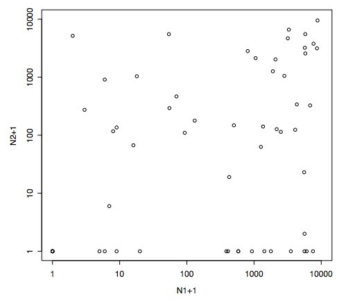
These results conform
to Tab. 1 in Couteron & Pélissier (2004), while
Fig. 1 is obtained from:
N1<-10000*smry$pvalsp[,1]
N2<-10000*smry$pvalsp[,2]
plot(N1,N2,log="xy",xlim=c(1,10000),ylim=c(1,10000),xlab="N1+1",ylab="N2+1")
3 - Distance-related analysis of species diversity
short<-spadis(tab~topo/xy,CFI,c("min",1),nrepet=10000)
short
#Contrast/Dissimilarity analysis
#class: spadis
#call: spadis(formula = tab ~ topo/xy, data = CFI, range = c("min", 1), nrepet
= 2)
#$mod: 1 2 (Two-way nested)
#distance range: (min,1]
#
#Summary table: tests based on 10000 distance permutations
#
P Pr Pr(>Pr)
#Richness 5.210 0.23600 0.998
#Shannon 0.326
0.01600 1.000
#Simpson 0.104
0.00515 1.000
#
# data.frame nrow ncol
content
#1 $spdis 59 3 by-species
range-related contrasts
long<-spadis(tab~topo/xy,CFI,c(5,"max"),nrepet=10000)
long
#Contrast/Dissimilarity analysis
#class: spadis
#call: spadis(formula = tab ~ topo/xy, data = CFI, range = c(5, "max"), nrepet
= 2)
#$mod: 1 2 (Two-way nested)
#distance range: (5,max]
#
#Summary table: tests based on 2 distance permutations
#
P Pr Pr(>Pr)
#Richness 5.210 2.4700 0.0133
#Shannon 0.326
0.1510 0.0048
#Simpson 0.104
0.0478 0.0098
#
# data.frame nrow ncol
content
#1 $spdis 59 3 by-species
range-related contrasts
Notice that observed values of P
and Pi are consistent with the values
in section 2.
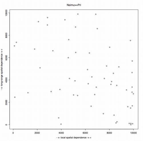
Results in Couteron
& Pélissier (2004) can
be summarized as follow:
Nshort<-10000*short$spdis[,3]
Nlong<-10000*long$spdis[,3]
plot(Nshort,Nlong,main="Nsimu>=Pri",xlab="- <- local
spatial dependence -> +",ylab="- <- long-range spatial dependence ->
+")
Variograms of dissimilarity are computed separately for uplands (hilltops, upper- and middle-slopes) and bottom-lands (thalwegs and foot-slopes; see Couteron et al. 2003):
topoS<-as.numeric(CFI$topo)
topoS[as.numeric(CFI$topo)<8]<-1
topoS[as.numeric(CFI$topo)>7]<-2
topoS<-as.factor(topoS)
uplands<-variodis(df=CFI$tab[topoS==1,],coords=CFI$xy[topoS==1,],breaks="Log",nrepet=300,alpha=0.1)
uplands
#Distance-related dissimilarity
analysis
#class: diversity
vario
#call: variodis(df=CFI$tab[topoS==1,],coords=CFI$xy[topoS==1,],breaks="Log",nrepet=300,alpha=0.1)
#
#10 % bilateral
CI computed from 300 distance permutations
#
# data.frame
nrow ncol content
#1 $richness
15 3 variogram of dissimilarity
#2 $Shannon
15 3 variogram of dissimilarity
#3 $Simpson
15 3 variogram of dissimilarity
#
# vector
length mode content
#1 $h
15 numeric distance
#2 $w
15 numeric bins weigths
Draw the variograms with
elimination of the low-weighted bins
plot(uplands,xlim=c(uplands$h[1],uplands$h[13])

bottomlands<-variodis(df=CFI$tab[topoS==2,],coords=CFI$xy[topoS==2,],breaks="Log",nrepet=300,alpha=0.1)
bottomlands
#Distance-related dissimilarity
analysis
#class: diversity
vario
#call: variodis(df=CFI$tab[topoS==2,],coords=CFI$xy[topoS==2,],breaks="Log",nrepet=300,alpha=0.1)
#
#10 % bilateral
CI computed from 300 distance permutations
#
# data.frame
nrow ncol content
#1 $richness
15 3 variogram of dissimilarity
#2 $Shannon
15 3 variogram of dissimilarity
#3 $Simpson
15 3 variogram of dissimilarity
#
# vector
length mode content
#1 $h
15 numeric distance
#2 $w
15 numeric bins weigths
Draw the variograms with
elimination of the low-weighted bins

Couteron, P., Pélissier, R. Mapaga, D., Molino, J.-F. and Teillier, L. 2003. Drawing ecological insights from a management-oriented forest inventory in French Guiana. Forest Ecology and Management, 172:89-108
Couteron,
P. and Pélissier, R. 2004. Additive apportioning of species diversity:
towards more sophisticated models and analyses. Oikos, 107(1):215-221.