Worked example 2 illustrates the use
of Diversity.R functions to perform
multivariate analyses that are consistent with diversity measurements, the
CA-richness and NSCA-Simpson strategies from Pélissier
et al. (2003). It is based on analyses of PSE data set,
from a 10-ha rainforest plot at Piste de St-Elie station (PSE) in French
Guiana (Sabatier et al. 1997).
1 -
PSE data set
Oncethe library diversity
has been installed and loaded:
PSE$Tfac is a factor of 113 species names
assigned to 381 trees ; PSE$Sfac is a factor of 9 soil classes
assigned to 381 trees ; PSE$Qfac is a factor of 80 quadrat codes
assigned to 381 trees.
2 - CA-richness and NSCA-Simpson
strategies with respect to the soil classes
Use the following commands
to perform a CA-richness strategy with respect to the soil classes: rich.sol<-ca.richness(PSE$Tfac~PSE$Sfac) #Select the number of axes:
2
summary(rich.sol)
#class: div between dudi
#metric: Richness
#call: ca.richness.formula(formula = PSE$Tfac ~ PSE$Sfac)
#total diversity: 112
#explained diversity: 2.33
#ratio of explained diversity: 0.0208
#Pr(>ratio): 0.551 based on 999 replicates
plot(rich.sol)
Use the following commands to perform a NSCA-Simpson strategy with respect
to the soil classes: simp.sol<-nsca.simpson(PSE$Tfac~PSE$Sfac) #Select the number of axes: 2 summary(simp.sol) #class: div between dudi #metric: Simpson #call: nsca.simpson.formula(formula = PSE$Tfac
~ PSE$Sfac) #total diversity: 0.933 #explained diversity: 0.0375 #ratio of explained diversity: 0.0402 #Pr(>ratio): 0.001 based on 999 replicates
3 - CA-richness and NSCA-Simpson strategies with respect to the partition
into quadrats
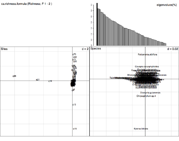
Use the following commands to perform a CA-richness strategy with respect
to quadrats:
rich.quad<-ca.richness(PSE$Tfac~PSE$Qfac)
#Select the number of axes: 2
summary(rich.quad) #class: div between dudi #metric: Richness #call: ca.richness.formula(formula = PSE$Tfac
~ PSE$Qfac) #total diversity: 112 #explained diversity: 23.6 #ratio of explained diversity: 0.211 #Pr(>ratio): 0.301 based on 999 replicates
plot(rich.quad)
Projection of the soil classes at the weigthed mean position
of their occurrences (as in Fig.4a in Pélissier
et al. 2003) can be obtained from:
Use the following commands to perform a NSCA-Simpson strategy with respect
to quadrats:
simp.quad<-nsca.simpson(PSE$Tfac~PSE$Qfac) #Select
the number of axes:
2
summary(simp.quad) #class:
div between dudi #metric: Simpson #call: nsca.simpson.formula(formula
= PSE$Tfac ~ PSE$Qfac) #total diversity:
0.933 #explained diversity:
0.214 #ratio of explained
diversity: 0.229 #Pr(>ratio):
0.001 based on 999 replicates
plot(simp.quad)
Projection of the soil classes at the weigthed mean position of their occurrences
(as in Fig.4b in Pélissier et al. 2003) can
be obtained from:
Sabatier, D., Grimaldi, M.,
Prévost, M.-F. , Guillaume, J., Godron, M., Dosso, M. and Curmi, P. 1997. The influence of soil cover
organization on the floristic and structural heterogeneity of a Guianan rain
forest. Plant Ecology, 131:81-108